hello algorithm chapter 2 / time complexity
Reference: Hello 算法 - 时间复杂度
Overview
- time complexity
- Definition
- Trend of algorithm running time
- The essence of analysis of time complexity is finding an asymptotic upper bound on the 'number of operations function'.
- Deductive method
- Ignore the constant terms
- Omit all coefficients.
- Use multiplication when nesting loops.
- judge asymptotic upper bound
- Common Time-Complexity
- O(1) < O(logn) < O(n) < O(nlogn) < O(n^2) < O(2^n) < O(n!)
- constant order
- linear order: single-layer loops
- square order: nested loops.
- exponential order
- recursive functions
- exhaustive methods (brute force search, backtracking, etc.).
- logarithmic order
- recursive functions
- divide-and-conquer strategy
- linear logarithmic order
- nested loops
- mainstream sorting algorithms, such as quicksort, merge sort, heapsort, etc.
- factorial order
- recursion functions
- total permutation
- Worst, Best, Average time complexity.
- we usually use the worst time complexity as a criterion for the efficiency of the algorithm.
Trend of algorithm running time
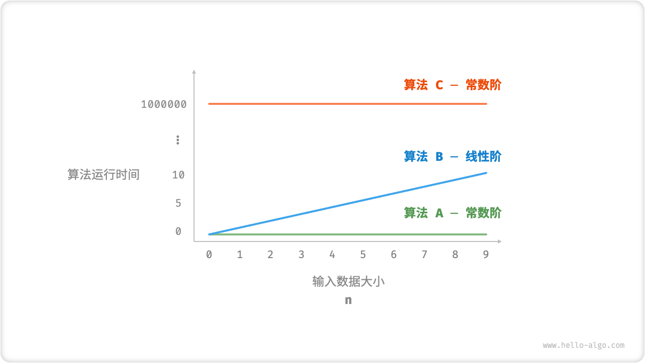
算法运行时间随着数据量变大时的增长趋势 = 时间复杂度
The growth trend of algorithm running time as the amount of data becomes larger = time complexity
Code for Algorithms
1 | |
Algorithm A and algorith C are both constant order. There are no difference between algorithm A and algorithm C.
Algorithm B is linear order.
Positive
- more efficient
- More convenient
Negative
- we can not judge time usage of algorithm depending on time complexity only.
Asymptotic upper bound
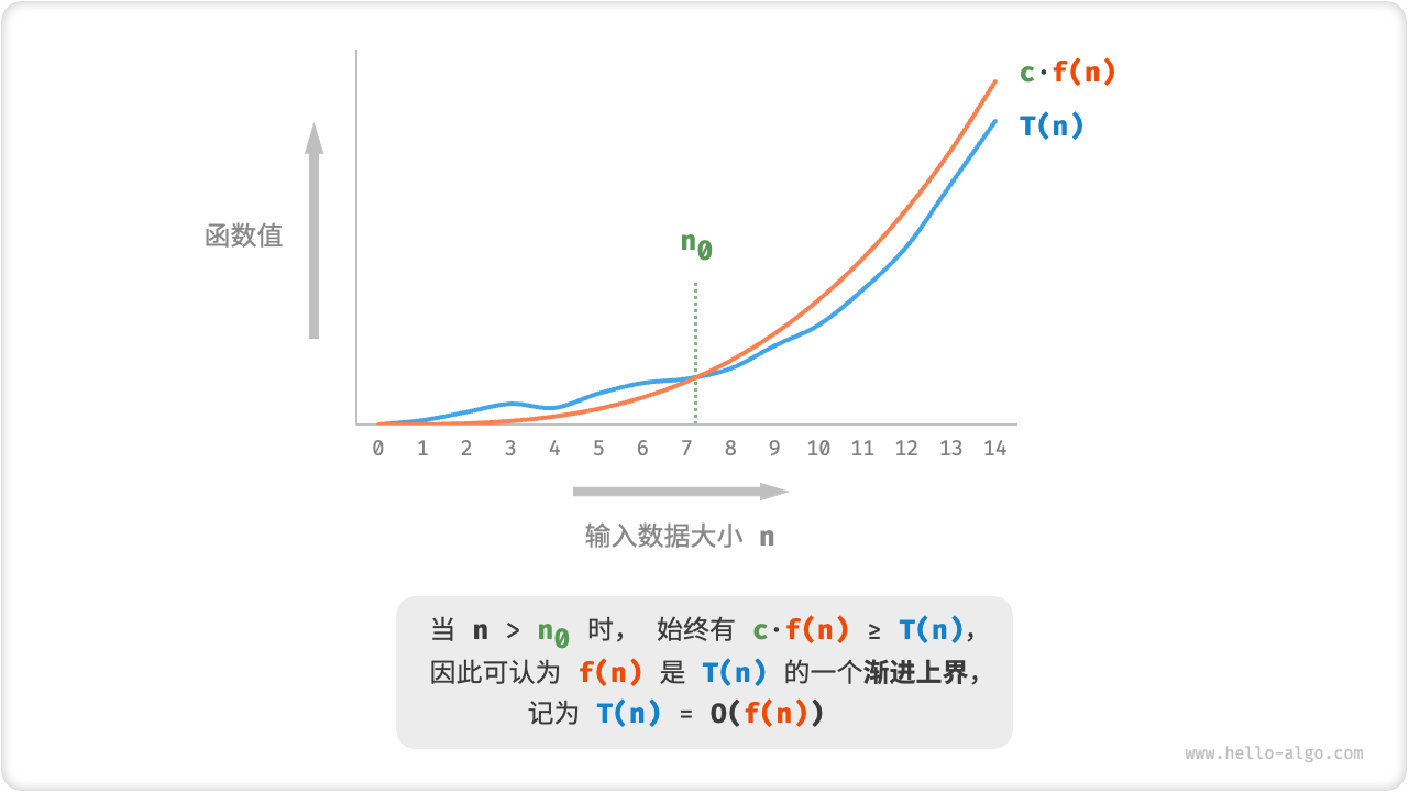
Assume that the number of operations of the algorithm is a function of the input data size \(n\), recorded as \(T(n)\).
The essence of analysis of time complexity is finding an asymptotic upper bound on the "number of operations function"
So, what is asymptotic upper bound?
If there are positive real numbers \(c\) and real numbers \(n_0\), such that for all \(n > n_0\), \(T(n) < c \times f(n)\), then \(f(n)\) can be considered as an asymptotic upper bound of \(T(n)\), Marked as \(T(n)=O(f(n)\)).
Deductive method
Step 1. statistics operation number
- Ignore the constant terms in \(T(n)\).
- Omit all coefficients. For example, loop \(2n\) times, loop \(5n+1\) times, etc. can be simplified and recorded as \(n\) times.
- Use multiplication when nesting loops. The total number of operations is equal to the product of the number of operations in the outer loop and the inner loop.
\(T(n)=2n + 1 + n^2\) equals \(T(n) = n + n^2\)
Step 2. judge asymptotic upper bound
The time complexity is determined by the term of the highest order in the polynomial. Cause that the term of the highest order will play a dominant role as it approaches infinity, the effects of all other terms can be ignored.
For exmaple, \(T(n) = n + n^2\) and \(O(T(n)) = O(n(^2))\).
Common Time-Complexity
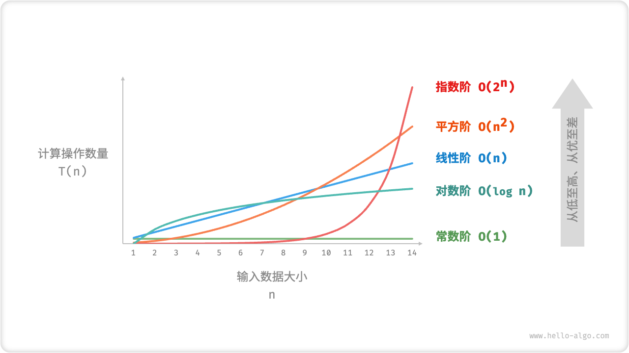
\(O(1) < O(logn) < O(n) < O(nlogn) < O(n^2) < O(2^n) < O(n!)\)
Constant order < logarithmic order < linear order < linear logarithmic order (线性对数阶) < square order < exponential order (指数阶) < factorial order (阶乘阶)
constant order
The number of operations of the constant order is independent of the input data size \(n\), that is, does not change with the change of \(n\).
Following function contain a loop, but time-complexity is \(O(1)\).
1 | |
linear order
The number of operations of linear order function grows in linear order relative to the size of the input data.
Linear order usually occurs in single-layer loops.
1 | |
square order
Square order usually occurs in nested loops.
1 | |
exponential order (指数阶)
In practical algorithms, exponential order often occurs in recursive functions.
在实际算法中,指数阶常出现于递归函数中。
For example, in the following code, it recursively splits in two and stops after a second split:
例如,在下面的代码中,它递归地分成两段,并在第二次分裂后停止:
1 | |
Exponential growth is very rapid and is more common in exhaustive methods (brute force search, backtracking, etc.).
指数阶增长非常迅速,在穷举法(暴力搜索、回溯等)中比较常见。
For problems with large data sizes, exponential order is not acceptable and usually needs to be solved using algorithms such as dynamic programming or greed.
对于数据规模较大的问题,指数阶是不可接受的,通常需要使用动态规划或贪心等算法来解决。
logarithmic order
In contrast to the exponential order, the logarithmic order reflects the situation where "each round is reduced to half."
与指数阶相反,对数阶反映了“每轮缩减到一半”的情况。
Let the input data size be \(n\), since each round is reduced to half, the number of cycles is the inverse function of, i.e.
设输入数据大小为 \(n\),,由于每轮缩减到一半,因此循环次数是 \(log_2n\), 即 \(2^n\) 的反函数。
1 | |
Similar to exponential order, logarithmic order is often found in recursive functions.
与指数阶类似,对数阶也常出现于递归函数中。
The following code forms a recursive tree with a height of \(n\):
以下代码形成了一个高度为 \(n\) 的递归树:
1 | |
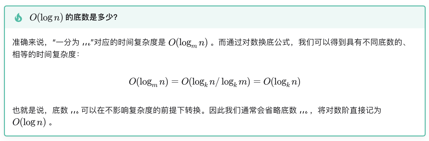
Logarithmic order often appears in the algorithm based on divide-and-conquer strategy, which reflects the algorithmic thought of "one is divided into many" and "making complex into simple".
对数阶常出现于基于分治策略的算法中,体现了“一分为多”和“化繁为简”的算法思想。
It grows slowly and is the ideal time complexity after constant order.
它增长缓慢,是仅次于常数阶的理想的时间复杂度。
linear logarithmic order (线性对数阶)
The linear logarithmic order often occurs in nested loops, and the time complexity of the two layers is \(O(n)\) and \(O(log_2n)\), respectively.
线性对数阶常出现于嵌套循环中,两层循环的时间复杂度分别为 \(O(n)\) 和 \(O(log_2n)\)。
1 | |
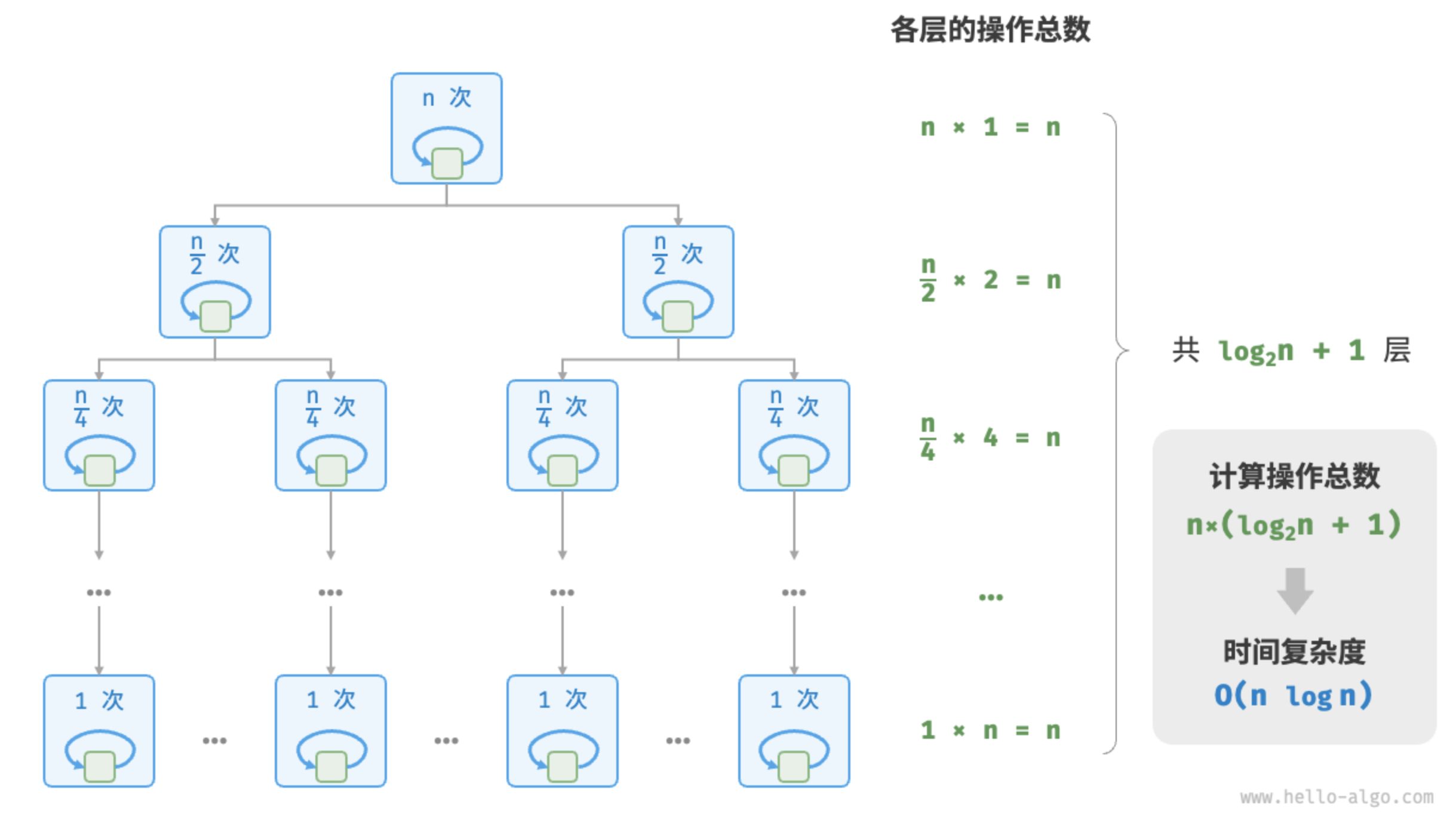
Follow graph show the process of generation of linear logarithmic order.
下图显示了线性对数阶的生成过程。
The total number of operations at each layer of the binary tree is \(n\), and the tree has \(log_2 n + 1\) layers, so the time complexity is \(O(nlogn)\).
二叉树的每一层的操作总数都为 \(n\),树共有 \(logn\) 层,因此时间复杂度为 \(O(nlogn)\)。
The time complexity of mainstream sorting algorithms is \(O(nlogn)\) usually, such as quicksort, merge sort, heapsort, etc.
主流排序算法的时间复杂度通常为 \(O(nlogn)\),例如快速排序、归并排序、堆排序等。
factorial order (阶乘阶)
The factorial order corresponds to the "total permutation" problem in mathematics.
阶乘阶对应数学上的“全排列”问题。
Given a non-repeating element \(n\), find all possible permutations of it, the number of schemes is:
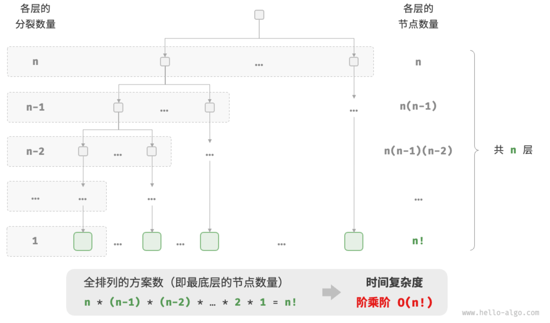
给定 \(n\) 个互不重复的元素,求其所有可能的排列方案,方案数量为: \[ !n = n \times (n-1) \times (n-2) \times ... \times 2 \times 1 \] Factorial is usually implemented using recursion.
阶乘通常使用递归实现。
As shown in Figure 2-14 and the following code, the first layer splits, the second layer splits, and so on until the first layer stops splitting:
如图 2-14 和以下代码所示,第一层分裂出 \(n\) 个,第二层分裂出 \(n-1\) 个,以此类推,直至第 \(n\) 层时停止分裂:
1 | |
$ n! > 2^n$ when \(n >= 4\). Therefore the factorial order grows faster than the exponential order, which is also unacceptable at large \(n\).
因为当 \(n >= 4\) 时恒有 $ n! > 2^n$ ,所以阶乘阶比指数阶增长得更快,在 \(n\) 较大时也是不可接受的。
Worst, Best, Average time complexity
The time efficiency of an algorithm is often not fixed, but is related to the distribution of the input data
算法的时间效率往往不是固定的,而是与输入数据的分布有关
The "worst time complexity" corresponds to the asymptotic upper bound of the function, which is represented by the large \(O\)notation.
“最差时间复杂度”对应函数渐近上界,使用大 \(O\) 记号表示。
Accordingly, the "best time complexity" corresponds to the asymptotic lower bound of the function, denoted by the token \(\Omega\).
相应地,“最佳时间复杂度”对应函数渐近下界,用记号 \(\Omega\) 表示。
The worst time complexity is more practical because it gives a safe value for efficiency.
而最差时间复杂度更为实用,因为它给出了一个效率安全值。
The worst or best time complexity occurs only in "special data distributions", which may be very rare and do not truly reflect the efficiency of the algorithm.
最差或最佳时间复杂度只出现于“特殊的数据分布”,这些情况的出现概率可能很小,并不能真实地反映算法运行效率。
In contrast, average time complexity represents the efficiency of an algorithm with random input data and is represented by the \(\Theta\)notation.
相比之下,平均时间复杂度可以体现算法在随机输入数据下的运行效率,用 \(\Theta\) 记号来表示。
For more complex algorithms, it is often difficult to calculate the average time complexity because it is difficult to analyze the overall mathematical expectation under the data distribution.
对于较为复杂的算法,计算平均时间复杂度往往是比较困难的,因为很难分析出在数据分布下的整体数学期望。
In this case, we usually use the worst time complexity as a criterion for the efficiency of the algorithm.
在这种情况下,我们通常使用最差时间复杂度作为算法效率的评判标准。
本博客所有文章除特别声明外,均采用 CC BY-SA 4.0 协议 ,转载请注明出处!